How To Set Up A Pivot Table / Pivot Table With Text In Values Area Excel Tips Mrexcel Publishing : Once the entire table is selected, go to the ribbon above in your excel and click on the insert tab.. Change the table/range value to the required cell range where your data set is placed. How to group pivot table dates. Click insert along the top navigation, and select the pivottable icon. If you are using excel 2003 or earlier, click the data menu and select pivottable and pivotchart report. Highlight your cells to create your pivot table.
You can apply value filtering on pivot tables to show just the top performing customer (or product, city etc.). This enables us to analyze, summarize, calculate, and visualize trends, comparisons, and patterns in our data.the steps below will walk through the process of grouping pivot table data by year. To set top 1 filter, simply click on the filter. To create a blank pivot table: Select the cells you want to create a pivottable from.
1 from Once the entire table is selected, go to the ribbon above in your excel and click on the insert tab. Ok, now we have everything we need to create our pivot table. While clicked inside a cell of the pivot table, visit the pivot table analyze tab of the ribbon, select the button for fields, items, and sets, and then click on calculated field. 2. How to group pivot table dates. To create a blank pivot table: Otherwise, you may run into errors or inaccuracies that misrepresent your data. Select the range of data for the pivot table and click on the ok button. Select the range of data for the pivot table and click on the ok button.
Once you've played around with the pivot table feature and gained some understanding of how the various options affect your data, then you can start creating a pivot table from scratch.
I changed the pivot table's name to sales. That pivottable's settings will be automatically imported and used in the future. Click insert along the top navigation, and select the pivottable icon. Click the insert tab at the top of the excel window. Select any of the cells from your pivot table. We can use a pivottable to group a set of data by year. While any large set of data can be turned into a pivot table, it's important to prepare your excel data for pivottables analysis in advance. I'm going to show you three months of dummy data first so you see what the pivot table is made of. To do so, highlight your entire data set (including the column headers), click insert on the ribbon, and then click the pivot table button. A create pivottable window should appear. Select the range of data for the pivot table and click on the ok button. You can apply value filtering on pivot tables to show just the top performing customer (or product, city etc.). Click any single cell inside the data set.
A create pivottable window should appear. How to insert and setting up pivot table in excel. While any large set of data can be turned into a pivot table, it's important to prepare your excel data for pivottables analysis in advance. Set up the pivot table's sales.numrows range. Select the range of data for the pivot table and click on the ok button.
Create A Pivottable To Analyze Worksheet Data Office Support from img-prod-cms-rt-microsoft-com.akamaized.net A create pivottable window should appear. Select the cells you want to create a pivottable from. That pivottable's settings will be automatically imported and used in the future. Your data shouldn't have any empty rows or columns. Select any cell within the data set. Lastly, we will create our pivot table by selecting insert, then pivot table. How to insert and setting up pivot table in excel. We can use a pivottable to group a set of data by year.
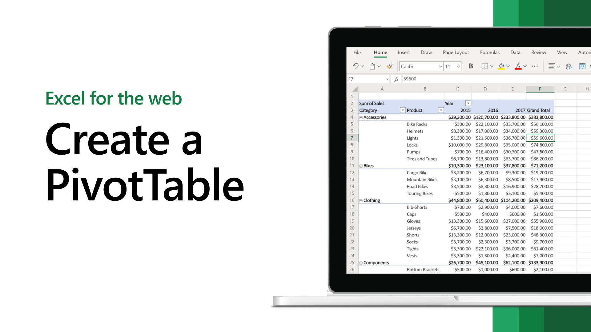
I added the text shown in cell a1 in the figure below.
Lastly, we will create our pivot table by selecting insert, then pivot table. I added the text shown in cell a1 in the figure below. How to insert and setting up pivot table in excel. Select the range of data for the pivot table and click on the ok button. Your data shouldn't have any empty rows or columns. Click insert along the top navigation, and select the pivottable icon. Enjoy this video of me guiding my viewers on how to create a pivot table with great ease! Click the insert tab at the top of the excel window. Highlight your cells to create your pivot table. In the tables group, click on the tables button and select pivottable from the popup menu. That pivottable's settings will be automatically imported and used in the future. I'm going to show you three months of dummy data first so you see what the pivot table is made of. This is the source data you will use when creating a pivot table.
Your source data should be setup in a table layout similar to the table in the image below. The first step to creating a pivot table is setting up your data in the correct table structure or format. In the tables group, click on the tables button and select pivottable from the popup menu. It will display the value of one item (the base field) as the percentage of another item (the base item).this option will immediately calculate the percentages for you from a table filled with numbers such as sales data, expenses, attendance. Go to the ribbon and select the insert tab.
How To Create A Pivot Chart In Excel from cdn.planacademy.com Ok, now we have everything we need to create our pivot table. Click insert along the top navigation, and select the pivottable icon. This will greatly reduce the size of your pivot table. Follow these instructions to ensure your pivot table will produce the results you are looking for. Once the entire table is selected, go to the ribbon above in your excel and click on the insert tab. Once you've played around with the pivot table feature and gained some understanding of how the various options affect your data, then you can start creating a pivot table from scratch. I added the text shown in cell a1 in the figure below. Select any cell within the data set.
Click ok to close the dialog box.
Highlight your cells to create your pivot table. Click insert along the top navigation, and select the pivottable icon. First, i inserted several rows above the pivot table. If you are using excel 2003 or earlier, click the data menu and select pivottable and pivotchart report. Once the entire table is selected, go to the ribbon above in your excel and click on the insert tab. But first, i needed to set up a formula that returns the number of rows in the pivot table. I added the text shown in cell a1 in the figure below. Click any single cell inside the data set. From the insert tab, choose to insert a pivot table. select the pivot table fields such as salesperson to the rows and q1, q2, q3, q4 sales to the values. To insert a pivot table, execute the following steps. I changed the pivot table's name to sales. While any large set of data can be turned into a pivot table, it's important to prepare your excel data for pivottables analysis in advance. This action will prompt another window, which will show you some options about where you would like to place your pivot table.